I. Discovery of Satellite Data Through a STAC Catalog
1. Introduction
1.1. Satellite data access: the emergence of cloud native solutions
There are several possibilities to discover and download satellite images. In a fairly classic way, we discover and download the images on websites. If we take the example of data from the Sentinel constellation, we connect to the SchiHub website of the Copernicus program.
However, there are other recent solutions based on new specifications. They make it possible to optimize in particular the download by targeting only the useful portions of the images.
This first notebook introduces the STAC (SpatioTemporal Asset Catalog) specification and outlines a practical and convenient method for searching and obtaining spatiotemporal assets.
Here we will use Microsoft’s Planetary Computer’s STAC Python API, but STAC is meant to be a standard that other data providers can adhere to.
We will also the following topics and operations which are relevant to using a STAC Catalog:
GeoJSON objects
structure
displaying GeoJSON objects a map
calculating bounding boxes for a set of GeoJSON objects
Coordinate Systems
1.2. The STAC specification
The STAC specification actually encompasses 4 semi-independent specifications:
STAC Item
STAC Catalog
STAC Collection
(STAC API)
Note: The STAC API provides specification for a RESTful endpoint (which is how the Python library
pystacinteracts with servers in the background). This is not relevant to most GIS users and falls outside the context of these notebooks.
The Item, Catalog and Collection specifications describe JSON objects with specific fields. Any JSON object that contains all the required fields for an Item (resp. Catalog, Collection) is a valid STAC Item (resp. Catalog, Collection). These JSON objects themselves do not contain any data, they store only metadata and links (more precisely URIs) to the data.
STAC Items are the smallest unit of the STAC specification. An Item represents one or several spatiotemporal assets. A STAC Catalog object is simply a group of other Catalog, Collection, and Item objects. STAC Collections are catalogs which describe a group of related items and thus they also contain dedicated metadata for those items.
2. Library imports
To start, we will first import several libraries that will be useful for the rest of this exercise:
pystac_client: package for working with STAC Catalogs and APIs that conform to the STAC and STAC API specs in a seamless waydinamis_sdk: package for working with MTD’s CDSpandas/geopandas: package that provides fast, flexible, and expressive (geo)data structures designed to make working with “relational” or “labeled” data both easy and intuitiveshapely: package for handling geospatial vector datafolium: package for visualizing spatial data via an interactive leaflet mapnumpy: the fundamental package for scientific computing in Python... and some other tools...
# library for handling STAC data
import pystac_client

# library for acessing Microsoft Planetary Computer's STAC catalog
import teledetection

# dataframes and their geospatial data counterpart
import pandas as pd
import geopandas as gpd

# library for vector data
import shapely

# visualization
import folium  # maps

# NumPy arrays
import numpy as np

# miscellanous
from IPython.display import display
import json
from functools import partial
from itertools import cycle
3. Handling GeoJSON layers
As mentioned above, STAC is fundamentally built as an extension of the GeoJSON format, hence it makes sense to first take a moment to look at this format.
3.1. GeoJSON structure
Here is an example of a simple GeoJSON Feature describing a rectangle Polygon: the geometry property and its coordinates sub-property are the most important, they contain the coordinates of the vertices of the polygon.
{
    "type": "Feature",
    "geometry": {
        "type": "Polygon",
        "coordinates": [
            [
                [4.825087, 43.949066],
                [4.919379, 43.949066],
                [4.919379, 43.885034],
                [4.825087, 43.885034],
                [4.825087, 43.949066],
            ]
        ],
    },
}
For a slightly more elaborate, we will use a GeoJSON collection of features made up of several Polygons. In this case there are 12 rectangles corresponding to different land cover classifications around the city of Montpellier, France.
with open("sample.geojson") as file:
    features = json.load(file)

print(f"the geoJSON type is: {features['type']}\n")
print("Example of geoJSON strcuture for the first feature:\n")
print(json.dumps(features["features"][0], indent=4))Exercise: Write a loop to obtain the list of land cover types.
# to fill
# ...
# ...
3.2 Displaying GeoJSON features on a map
Here, we use Folium package to display the geometries of GeoJSON features through an interactive map.
The first block of code is dedicated to some formattig settings:
# configuring some formatting settings for the map visuals
higlight_fn = lambda x: {"fillOpacity": 0.5}
FGJSON = partial(folium.GeoJson, highlight_function=higlight_fn, zoom_on_click=True)

colors = cycle(["green", "grey", "orange", "red", "yellow", "purple", "pink", "brown"])
style_fn = lambda x: {"color": next(colors), "fillOpacity": 0}
Here is the main part for displaying the GeoJSON features:
with open("sample.geojson") as file:
    features = json.load(file)

# We can use folium to easily visualize the polygons on a map
maps = folium.Map(location=[43.6085, 4.0053], zoom_start=11, control_scale=True)
polygon_group = folium.FeatureGroup(name="polygons").add_to(maps)

# these groups will only used later but it needs to be created before rendering the map
polygon_extent_group = folium.FeatureGroup(
    name="polygons extent", control=False
).add_to(maps)
sat_extent_group = folium.FeatureGroup(name="satellite extents", control=False).add_to(
    maps
)

maps.keep_in_front(polygon_group)
maps.add_child(polygon_group)
for feature in features["features"]:
    a = folium.GeoJson(feature["geometry"], name=feature["properties"]["landcover"])
    polygon_group.add_child(a)
folium.LayerControl().add_to(maps)

maps
3.3. Determining the bounding box of GeoJSON objects
Since we’re dealing with multiple polygons, having an additional polygon which covers the full extent will prove useful. Here we will use shapely to get the bounds of a MultiPolygon object. However simply looping on each polygon and keeping track of minimums and maximums of latitude and longitude is a completely valid alternative, if a little more involved.
from shapely.geometry import shape, MultiPolygon, box

# create a shapely MultiPolygon from each GeoJSON polygon
union = MultiPolygon(shape(feature["geometry"]) for feature in features["features"])
# create a new Polygon from the bounds of the union
extent = box(*union.bounds)

# export as a GeoJSON object
extent_geo_json = json.loads(shapely.to_geojson(extent))


fgjson = folium.GeoJson(
    extent_geo_json,
    highlight_function=lambda x: {"fillOpacity": 0},
    style_function=style_fn,
)
polygon_extent_group.add_child(fgjson)
polygon_extent_group.control = True

maps
4. Exploring a STAC catalog
We now want to list the Sentinel-2 images available on the previously calculated bounding box. Here, we will explore the Microsoft Planetary Computer catalog.
4.1. STAC architecture
4.1.1. STAC Catalog
STAC Catalog can simply be seen as a directory of other STAC objects (Catalogs, Collection and Items). There are very little restrictions placed on Catalogs, the way they’re organized tends to depend on the specific implementation.

STAC Collection Layout and Specification
Figure by https://
4.1.2. STAC Collection
STAC Collections are built upon STAC Catalogs. Collections are meant to group homogeneous data, so they include additional fields to describe the data, such as spatial and temporal extent, license and other metadata.

STAC Collection Specification
Figure by https://
4.1.3. STAC Item
STAC Item is built upon the GeoJSON specification. GeoJSON is a format for encoding different geometric data structures such as points, lines and polygons. It is widely used by standard geospatial libraries such as Shapely.
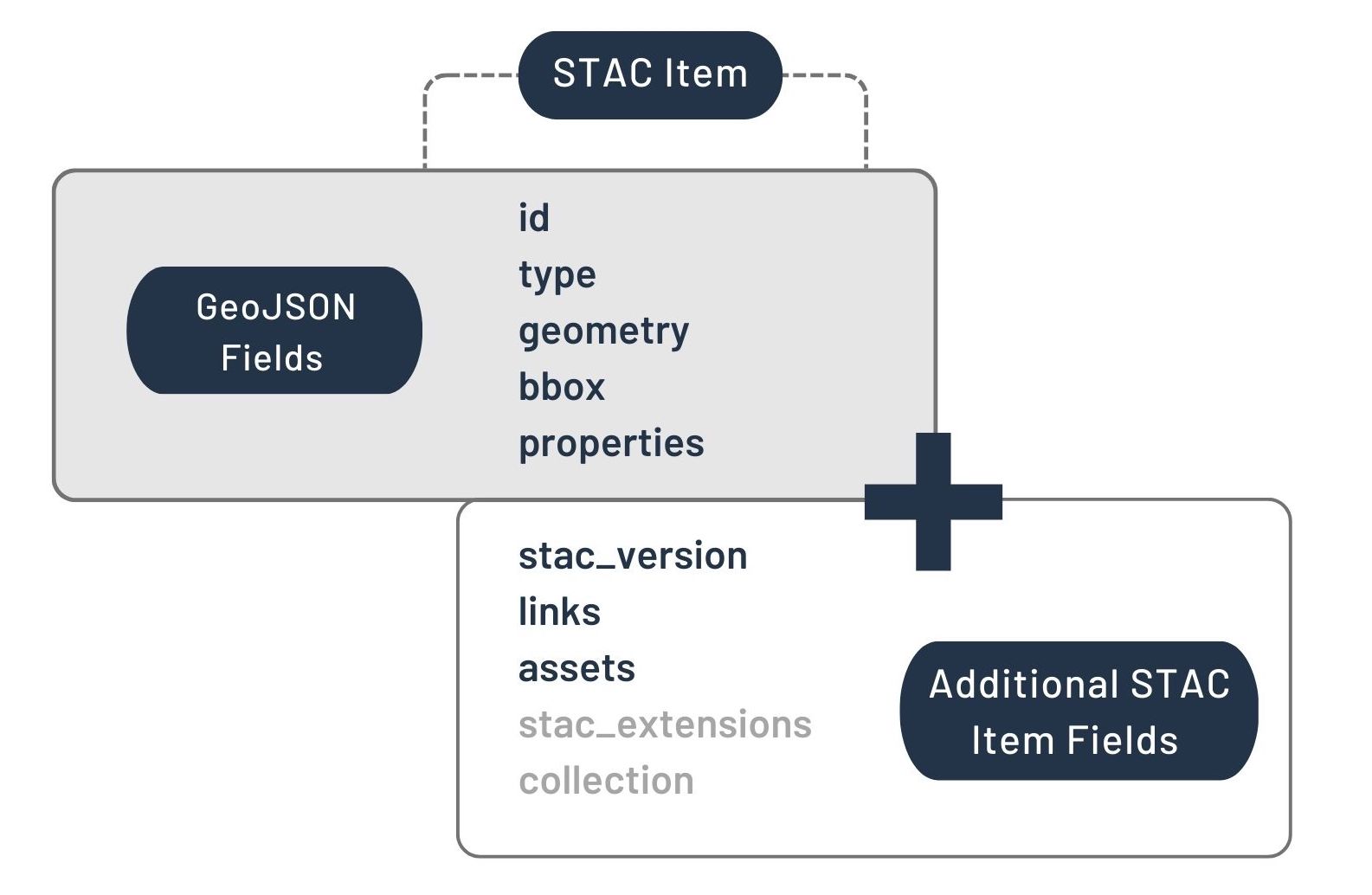
STAC Item Specification
Figure by https://
4.2. Opening CDOS’s STAC Catalog
4.2.1. CDOS API connection
Let’s start by opening a client object to the CDOS STAC catalog.
api = pystac_client.Client.open(
    "https://api.stac.teledetection.fr",
    modifier=teledetection.sign_inplace,
)

stac_item = api.get_collection("sentinel2-l2a-theia").get_item(
    "SENTINEL2A_20201203-104853-415_L2A_T31TEJ_D"
)
IMPORTANT: The URLs that we obtain from the STAC Catalog are not valid indefinitely. They expire after about 5 days. If you see an error in the notebook, it is likely because the URL that you obtained by running the first few cells has now expired. If that happens you should be able to just run the notebook again from the top to get a new URL. You can get longer-lasting URLs by registering an API key. More info here.
Most of the objects we will be using in this notebook include rich text formatting and some HTML. That means we can easily have a look at objects by using the display function of IPython.display or simply using the default output behavior of the last line of the cell in notebooks.
# These two next lines are equivalent
display(api)
api
Let’s have a look at the contents of the catalog object. This particular Catalog object we have created is the parent group of all the STAC objects that Planetary Computer provides.
As a reference here is a list of the fields defined in the STAC Catalog specification.
| Element | Type | Description |
|---|---|---|
| type | string | REQUIRED. Set to Catalog if this Catalog only implements the Catalog spec. |
| stac_version | string | REQUIRED. The STAC version the Catalog implements. |
| stac_extensions | [string] | A list of extension identifiers the Catalog implements. |
| id | string | REQUIRED. Identifier for the Catalog. |
| title | string | A short descriptive one-line title for the Catalog. |
| description | string | REQUIRED. Detailed multi-line description to fully explain the Catalog. CommonMark 0.29 syntax MAY be used for rich text representation. |
| links | [Link Object] | REQUIRED. A list of references to other documents. |
We can see that the catalog object does contain most of the required fields for a Catalog object. However it does not include the stac_version field, so it is not technically a completely valid Catalog object.
4.2.2. List of collections
Now let’s look at the Collection objects that are in catalog.
collections = [
    (collection.id, collection.title) for collection in api.get_collections()
]
pd.set_option("display.max_rows", 150)

pd.DataFrame(collections, columns=["Collection ID", "Collection Title"])
4.2.3. Exploring a Sentinel-2 collection
In the table above we can clearly see how each collection (i.e. each row) of Planetary Computer’s catalog corresponds to a dataset with common properties. Let’s now look at a collection in particular:
# We use the collection id from the table above to obtain the collection object
collection_name = "sentinel2-l2a-theia"
catalog_s2 = api.get_collection(collection_name)
catalog_s2
By reading the description field we can see that this collection contains all of the data from Sentinel-2 processed to L2A (bottom-of-atmosphere), ranging from 2016 to the present. It is obvious that looking through all this data in the same way that we did for the collections themselves would not be practical.
The simplest way to search through a catalog is to use the search method on a catalog object.
The important arguments for the search methods are the following:
collections: restricts the search to the collections whichidwere providedrestricting spatial extent using either:
bbox: simple bounding box given as [min(longitude), min(latitude), max(longitude), max(latitude)]intersects: GeoJSON object, or an object implementing a__geo_interface__property (supported by libraries such as Shapely, ARcPy, PySAL, geojson)
datetime: using adatetime.datetimeobject or a string. For a time range you can use'yyyy-mm-dd/yyyy-mm-dd'(beginning/end), or even'2017'as a shortcut for'2017-01-01/2017-12-31', and2017-06for the whole month of June 2017query: a list of JSON of query parameters. This allows to search for specific properties of items (such as cloud cover), and will be used in a later notebook
Note: Finding GPS coordinates can be as simple as going to google.com/maps and right clicking a point on the map. However, be careful that although standards dictate that coordinates should be given with latitude first and longitude second, some tools and libraries use longitude first and latitude second, often as a similarity to coordinates on a plane.
For now, let’s reuse the extent GeoJSON Polygon we created earlier.
# Here longitude comes first
area_of_interest = extent_geo_json
area_of_interest
The bbox parameter expects a Python list formatted as follows:
[xmin, ymin, xmax, ymax]So we have to modify area_of_interest in order to keep the right coordinates.
# Here is the equivalent bbox object to the polygon above
# using a numpy array for convenient axis operations
coords = np.array([area_of_interest["coordinates"]][0][0])
bbox = [*coords.min(0), *coords.max(0)]
bbox
Let’s use the following datetime format:
"start_date<yyyy-mm-dd>/end_date<yyyy-mm-dd>"time_range = "2020-12-01/2020-12-31"Now, we can search the Sentinel-2 images (i.e. STAC Items) that match our criteria. Here we present the two ways to pass the spatial query (bbox and intersects).
# the id for a collection can be found in the table we created earlier
collections = [collection_name]

# As expected the GeoJSON object and
# bounding box methods give the same results
search = api.search(collections=collections, datetime=time_range, bbox=bbox)
items = search.get_all_items()
print(f"{len(items)} items found with the `bbox` parameter")

search = api.search(
    collections=collections,
    datetime=time_range,
    intersects=area_of_interest,
)
items = search.get_all_items()
print(f"{len(items)} items found with the `intersects` parameter")
The result of a search is an ItemCollection, which is similar to the objects we’ve seen previously. Thus we can look through it just the same with display or Jupyter’s cell magic. We can then check that the results are from the right dataset (Sentinel-2 L2A), the right date ranges, and the geometry we specified falls within the specified bbox of each item.
display(items)The results of the search are STAC Item objects. Here each Item corresponds to an acquisition of Sentinel-2. Each Item contains Assets. In our case assets are satellite images. If we look through the assets of one of the search result, we see that each band corresponds to an asset, but we also have additional assets like the Scene classification map (SCL) which attempts to classify pixels within 12 classes (including No Data, defective pixel, cloud, snow or ice, vegetation, etc.). As mentioned previously, there is no data in an Asset object, only a link to the data (the href property).
One other thing to note is the STAC Extensions section. STAC is meant to be very general and does not make many assumptions to the nature of the data it describes. This is why STAC Extensions can be created to help extend the basic scheme. The items we obtained all implement three extensions:
eo: Electro-Optical Extension Specification which helps describe data that represents a snapshot of the Earth for a single date and timesat: Satellite Extension Specification which helps describe metadata related to a satelliteprojection: Projection Extension Specification which helps describe data related to the projection of GIS data (CRS, geometry, bbox, shape, etc.)
STAC extensions can be freely created, but most are released and described at https://
Exercise: search how many landsat images (collection: ‘landsat-c2-l2’) intersect our area of interest between 2020-12-01 and 2020-12-31.
# to fill
# ...
# ...
4.3 Coordinate systems
The GIS (Geographic Information System) field loves their acronyms. One such acronym is so ubiquitous that it is rarely explained: CRS. It refers to Coordinate Reference System. A CRS is a coordinate-based system used to locate geographical entities. The EPSG registry is a public registry of such coordinate systems. The GPS coordinates we’ve handled so far use are defined in a coordinate system which EPSG code is EPSG:4326. Since GPS coordinates are so widely known and available, they have become a de facto standard for geospatial data. In most situations, if a coordinate system is not specified it is safe to assume that coordinates are given in EPSG:4326.
Note: The EPSG database specifies the order of the axis. For instance (latitude, longitude) is the order of axis for EPSG:4326, with units going up in the north and east directions. However, as mentioned previously, some libraries and programs ignore this part of the standard. They instead choose (longitude, latitude) as their default.
For Planetary Computer itself, that standard becomes crucial. Even within a collection the CRS might not be the same. For example Sentinel-2 uses the Universal Transverse Mercator (UTM) system. This system divides the Earth into 60 zones of 6° of longitude in width. Furthermore, for a same UTM zone the CRS is also different in the northern and southern hemispheres. In total, depending on the location, Sentinel-2 data uses one of 120 different CRS! In order to permit searching with a bounding box or intersects, the bbox field of Items uses GPS coordinates, even if the underlying data uses a different coordinate system.
4.4 Finding the least cloudy image
4.4.1. Converting Items to GeoDataFrame
In some situations such as this one, it may be be more convenient to import the search result items into a dataframe (or table) with a library like geopandas. Here we see the crs parameter being used so that the geopandas knows which coordinate system is being used for the table. This would be crucial if we needed to change the coordinate system for our coordinates.
df = gpd.GeoDataFrame.from_features(items.to_dict(), crs="epsg:4326")
df
We can use the geometry property of the assets to visualize the extent of each satellite image.
extents = json.loads(df["geometry"].to_json())
for feature in extents["features"]:
    folium.GeoJson(feature["geometry"], style_function=style_fn).add_to(
        sat_extent_group
    )
sat_extent_group.control = True
maps
4.4.3. Filtering by cloud cover
As we’ve seen before, the 'sentinel-2-l2a' collection implements the eo extension (as indicated in the STAC extension section of the Item). This means we can use the eo:cloud_cover field to select the item (i.e. acquisition date) with the lowest cloudiness.
selected_item = min(items, key=lambda item: item.properties["eo:cloud_cover"])
print(
    f"The lowest cloudiness has a value of {selected_item.properties['eo:cloud_cover']} for date {selected_item.datetime}"
)
selected_item
4.4.4. The Item’s Assets
Finally let’s have a look at the assets for that item we selected.
values = [asset.title for asset in selected_item.assets.values()]
descriptions = pd.DataFrame(
    values,
    columns=["Description"],
    index=pd.Series(selected_item.assets.keys(), name="asset_key"),
)
descriptions
print(selected_item.assets["QL"].to_dict())
from IPython.display import Image
Image(url=selected_item.assets["QL"].href, width=500)Exercise: Display the least cloudy landsat image (preview).
# to fill
# ...
# ...